Pricing of a bet – Part 2 – The bet

This is the second thread on the theory behind the recently established Smarkets market on the prospects of a Conservative lead by end of January (covered here).
The first part presented the theory of this bet.
This part presents a simplified worked example and has a mathematical annex, following which:
- The next part will examine historic evidence on the volatility of opinion polls, which is an important input variable and interesting in itself
- The final thread will look at the possibility of serial autocorrelation in the change in Labour leads and its implications for the bet, and at the implications of there being more than one polling company.
Worked example – single poll
From the theory presented in the previous thread, it is trivial to work out the fair value of the bet, and hence the implied odds. I have done so in the table below.
| SD | Chance of a lead in the next poll | Approximateimplied odds |
| 3 | 3.4% | 30/1 |
| 2 | 0.3% | 300/1 |
| 1 | ~0% | >1,000/1 |
Worked example – multiple polls
However, the above example is only of use when there is a single poll left in the time period covered by the bet. Those interested can see the technical algebraic proof of the result for two polls in the Mathematical Annex below.
But what about when there are, say, six polls remaining?
The probability that a three-poll bet will be a loser is the probability that poll 1 AND poll 2 AND poll 3 show Conservative leads below 0.5%. Unfortunately, this is where the maths starts to get extremely complicated.
The proof for more than two polls runs to a dozen pages of dense algebra, so I have not reproduced it here.
Of more interest to the practical gamblers on this site, I have crunched the numbers using the Excel shortcut described in the previous thread to find the likelihood of winning for a given number of polls and for different standard deviations given a Labour lead of 5:
| Probability of winning after:Given: | 1 poll | 2 polls | 3 polls | 4 polls | 5 polls | 6 polls |
| SD=6 | 17.2% | 30.4% | 39.3% | 45.7% | 50.3% | 53.9% |
| SD=4 | 8.5% | 19.6% | 28.0% | 34.5% | 39.0% | 43.5% |
| SD=2 | 0.3% | 3% | 6% | 10% | 14% | 18% |
| SD=1 | <0.1% | <0.1% | 0.1% | 0.4% | 1% | 2% |
Conclusion
Anybody who has followed me this far will see how the probability of winning the bet depends on three inputs:
- the current Labour lead;
- the number of polls left in the bet; and
- the standard deviation of Labour’s lead.
We know, or can guess, the first two. However, the third, how much polls change over time, is much less certain.
It is the subject of the third part of this short series on the pricing of this bet.
Mathematical Annex
For t?1, we have:
Yt=Yt?1+Nt
Where Nt?N(0,SD2).
We suppose that Y0=a, the initial level of the lead. So Y1=a+N1 and Y2=Y1+N2=a+N1+N2.
Given a level of lead at which the bet is won, m, we aim to calculate P(Y1?m or Y2?m). This is given by 1?P(Y1< m,Y2< m). We can use the Bayesian formula for conditional probability to calculate the odds:
P(Y2< m|Y1< m) =P(Y1< m,Y2< m)P(Y1< m)
which gives
P(Y1< m,Y2< m) =P(Y2< m|Y1< m)P(Y1< m).
Since we know P (Y1< m), we just need to calculate the conditional probability.
Let phiY1(x) be the density function for Y1and phi(N2) the cumulative distribution function for N2. Then:
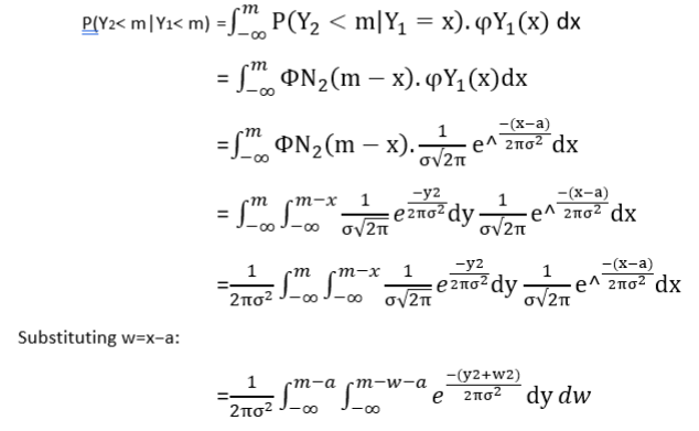
[Thanks to a couple of mathematically-inclined friends for helping with the above]